![]()
During my PhD, the majority of the work I did revolved around what is known as the Bayesian causal inference model of multisensory integration. This model has proven to be very successful in explaining many of the phenomena that human observers will exhibit when tested in many of the most commonly administered psychophysical tests of multisensory interactions. While the list of relevant publications is long, I’ll include just one of the more recent ones. I am referring to our 2015 publication “Perception of body ownership is driven by Bayesian sensory inference.”
As an alternative to the Coupling prior model (see my previous post showing my implementation of that), this model provides several key innovations, at the cost of added model complexity. In particular, the framework that underlies the Bayesian model affords greater conceptual clarity, being what we call a normative model that is derived from first principles. The model concerns itself with the causal structure of the objects “out there” in the real world that are deemed to be most likely to have generated the sensory stimuli that are now arriving to the nervous system. A quick side-by-side comparison of the two GUIs I have created here will show, however, the downside to this property, namely an almost two-fold increase in the number of parameters required to fully characterize the model. In contrast, the coupling prior model is a much simpler and more computationally convenient framework to use, and therefore more parsimonious. In short, that framework remains at the level of the stimulus space itself, and does not attempt to invoke inferences regarding the physical causal structure, but rather uses knowledge regarding the covariance structure between multimodal stimuli that has been accumulated across a lifetime of experience.
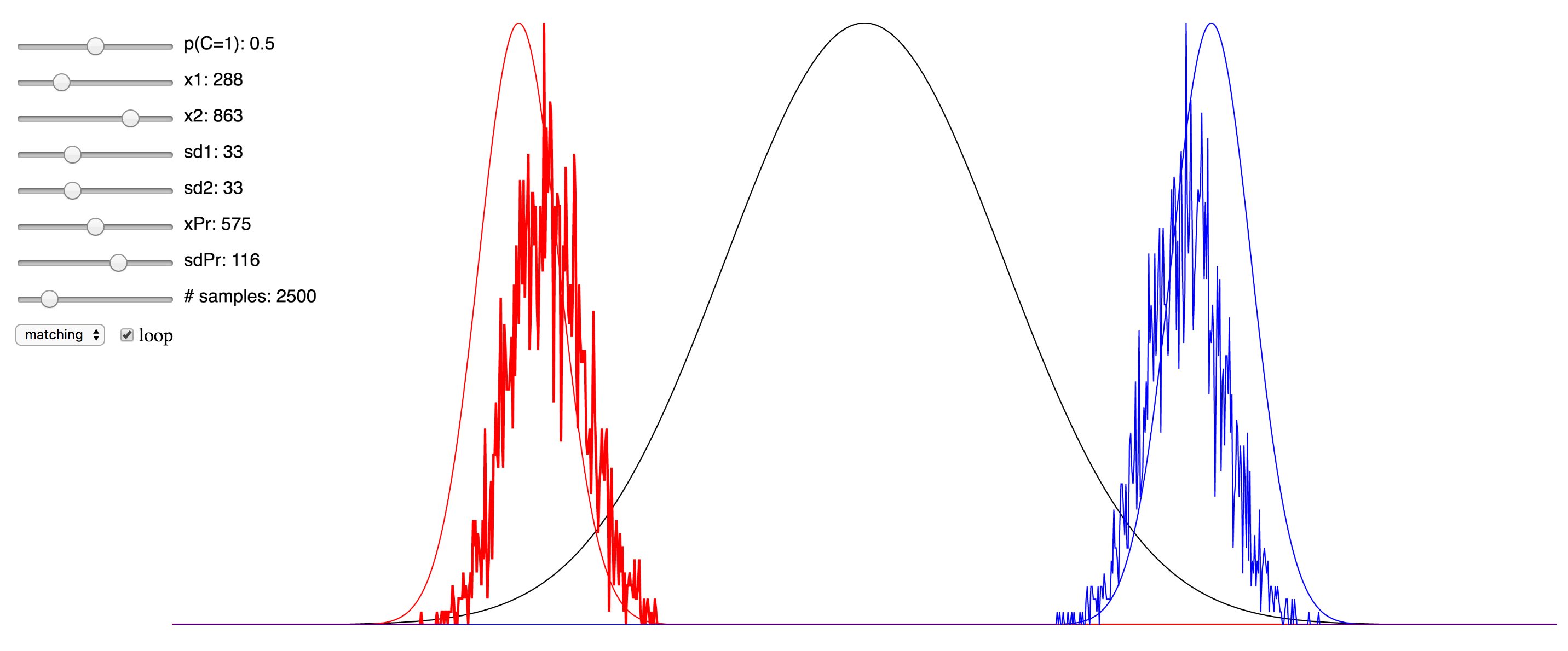
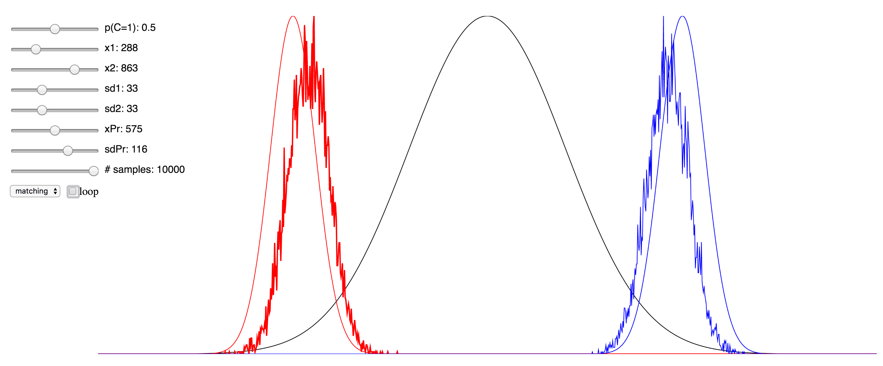
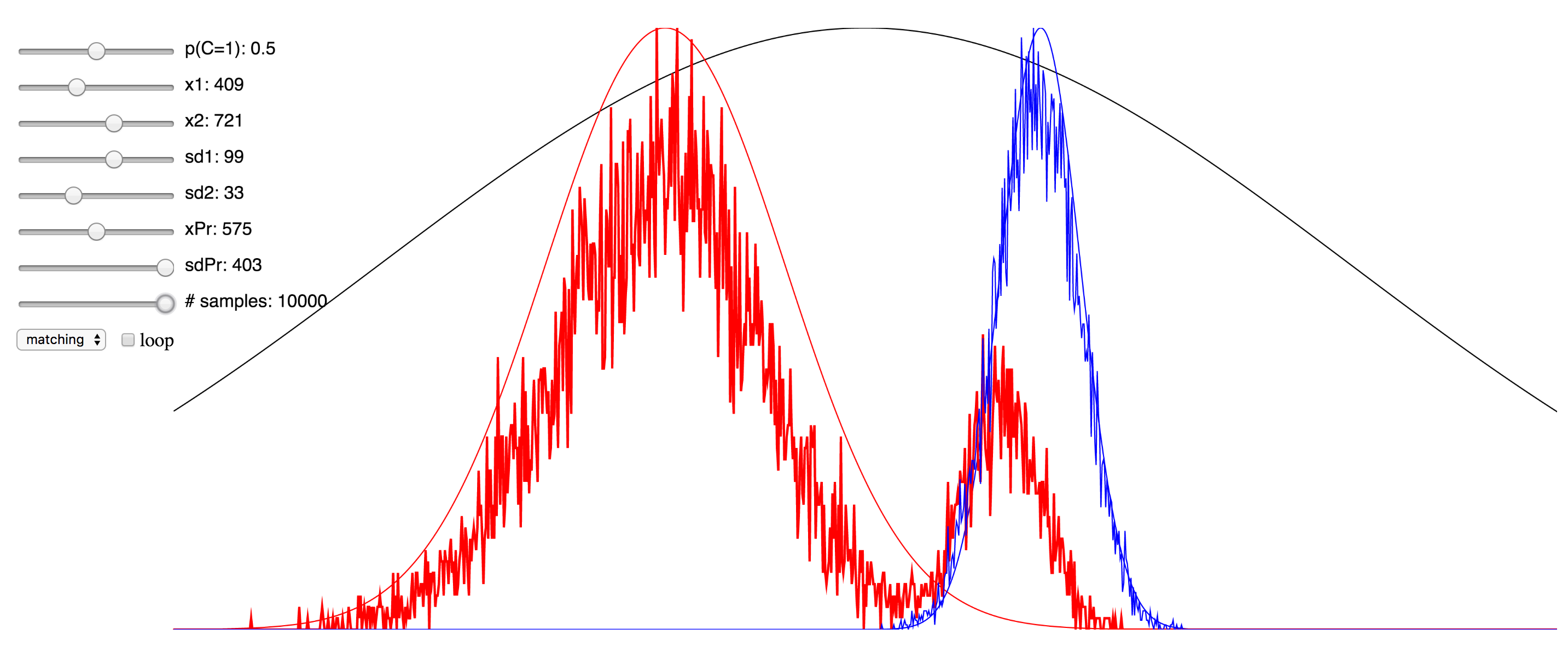
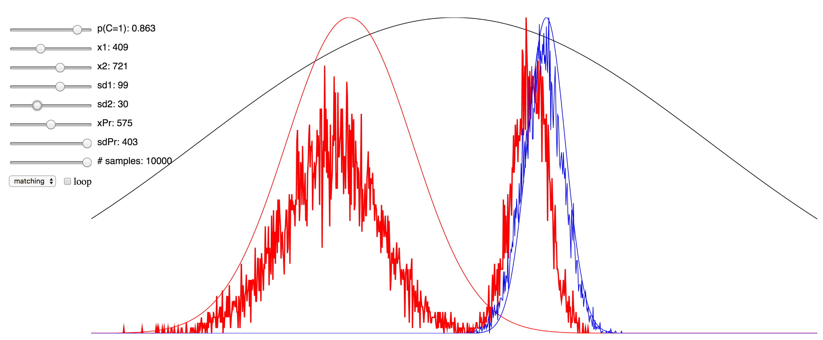
Regardless of the pros and cons of both approaches, I thought it might be instructive to the students of this field who are trying to learn about the various approaches to see a simulation that enables the setting of values for the different parameters and observing in real time the effect this has. To that end, I have ported over the Matlab implementation of the Bayesian causal inference model into JavaScript, making use of the p5.js framework, as well as this very helpful JS library for the Gaussian distribution.
Since I was not able to embed the live simulation that will run in the browser into this page, I have hosted it on my domain, and you can access it at here. I have also included a few screenshots of the simulation below. You can click on any of them to be taken to simulation. Note that if it starts to take up too much processor time, you can uncheck the “loop” checkbox to make it only evaluate after any change to the sliders, rather than in real-time. Also, try reducing the number of samples sliders to minimize the computational burden. There are probably several things I could have done to optimize this, but since I am not a web developer, I do not know them. My code is hosted here, and if anyone has any suggestions, please feel free to send me a pull request.